Contributions
- Introducing the VQ-VAE model combining the variational autoencoder (VAE) framework with discrete latent representations. The model is simple, does not suffer from “posterior collapse”, has no variance issues.
- VQ-VAE gets the similar performance as its continuous counterpartss, while offering the flexibility of discrete distributions. The author demonstrates the learning ability of VQ-VAE in unsupervised situations and its interesting applications.
VAES
- VAEs consist of the following parts: an encoder network which parameterises a posterior distribution $q(z|x)$ of discrete latent random variables $z$ given the input data $x$, a prior distribution $p(z)$, and a decoder with a distribution $p(x|z)$ over input data.
VQ-VAE Method
-
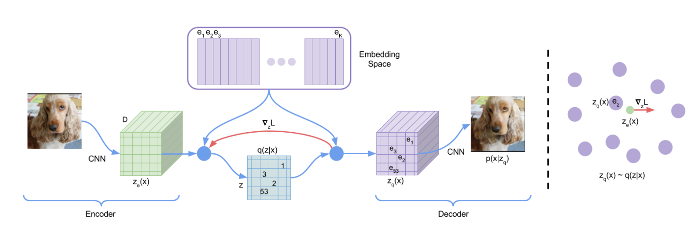
In VQ-VAE, the posterior and prior distributions are categorical, and the samples drawn from these distributions index an embedding table. These embeddings are then used as input into the decoder network.
-
Discrete Latent variables. Author defines a latent embedding space $e \in R^{K\times D}$ where $K$ is the size of the discrete latent space, and $D$ is the dimensionality of each latent embedding vector $e_i$. Thus, there are $K$ embedding vectors $e_i \in R^D, i \in \{1,2,…,K\}$.
-
Forward Process. VQ-VAE takes an input $x$, that is passed through an encoder producing output $z_e(x)$. The discrete latent variables $z$ are then calculated by a nearest neighbour look-up using the shared embedding space $e$ as shown in the following equation
\[q(z=k|x)=\left\{ \begin{aligned} 1, &\text { for k}=argmin_j\|z_e(x)-e_j\|_2\\ 0, &\text { otherwize} \end{aligned} \right.\]where $z_e(x)$ is the output of the encoder network.
The representation $z_e(x)$ is passed through the discretisation bottleneck followed by mapping onto the nearest element of embedding $e$
\[z_q(x)=e_k, \text{where }k=argmin_j\|z_e(x)-e_j\|_2\]The input to the decoder is the corresponding embedding matrix $z_q(x)$. One can see this forward computation pipeline as a regular autoencoder with a particular non-linearity that maps the latents to 1-of-K embedding vectors.
-
Backward Process. There is no real gradient defined in the quantization module. However, author approximate the gradient similar to the straight-through estimator and just copy gradients from decoder input $z_q(x)$ to encoder output $z_e(x)$. Since the output representation of the encoder and the input to the decoder share the same $D$ dimensional space, the gradients contain useful information for how the encoder has to change its output to lower the reconstruction loss.
The following equation specifies the overall loss function
\[L=log p(x|z_q(x))+\|sg[z_e(x)]-e\|_2^2+\beta \|z_e(x)-sg[e]\|^2_2\]where sg stand for the stopgradient operator and has zero partial derivatives.
There are three components that are used to train different parts of VQ-VAE. The first term is the reconstruction loss which optimizes the decoder and the encoder. Due to the straight-through gradient estimation of mapping from $z_e(x)$ to $z_q(x)$, the embeddings $e_i$ receive no gradients from the reconstruction loss $logp(z|z_q(x))$. Therefore, in order to learn the embedding space, the author uses the $l_2$ error to move the embedding vectors $e_i$ towards the encoder outputs $z_e(x)$ as shown in the second term of equation. Finally, since the volume of the embedding space is dimensionless, it can grow arbitrarily if the embeddings ei do not train as fast as the encoder parameters. To encourage the output of encoder to stay close to the chosen codebook vector to prevent it from flucturating too frequently from one code vector to another, author add a commitment loss, the third term in equation.
-
Prior. The prior distribution over the discrete latents $p(z)$ is a categorical distribution, and can be made autoregressive by depending on other $z$ in the feature map. Whilst training the VQ-VAE, the prior is kept constant and uniform. After training, we fit an autoregressive distribution over $z$, $p(z)$, so that we can generate $x$ via ancestral sampling.